Decision Trees in Python

Cover Photo By Marcelo Silva on Unsplash
Content Photo By The Sinking of the RMS Titanic, Nathan Walker

Prediction of Titanic Survivals with Decision Tree in Python
Modelling Questions

All models are wrong, but some are useful.

Did titanic survivals occur by chance? Or did they apply to the well known “survival of the fittest”? And what could that mean in a ship sank?
The goal of this project is to spot the features patterns that led to survival. We learn these patterns on train data given the ten predictors described below; then we predict the survival on test data and conclude with the evaluation of our model. This project was a good learning exercise for me since many questions emerged to my mind regarding predictive modelling and learning algorithm selections. How decision trees make decisions, is any one out there with better decision making skills, and how to find out the most accurate types of features(evidence) in decision making, are questions discussed in this note while the code is available in Python here.

Asking the Right Question:
“Use the Machine Learning Workflow to process and transform the titanic dataset to create a prediction model. This model must predict which passengers are likely to survive from the titanic sank with 90% or greater accuracy.”

Data description:

1. Survival - Survival (0 = No; 1 = Yes). Not included in test data.
2. Pclass - Passenger Class (1 = 1st; 2 = 2nd; 3 = 3rd)
3. Name - Name
4. Sex - Sex
5. Age - Age
6. Sibsp - Number of Siblings/Spouses Aboard
7. Parch - Number of Parents/Children Aboard
8. Ticket - Ticket Number
9. Fare - Passenger Fare
10. Cabin - Cabin
11. Embarked - Port of Embarkation (C = Cherbourg; Q = Queenstown; S = Southampton)

Selecting the proper algorithm and model

Model selection depends on the type of data we are analyzing and the output we predict. Model selection and output validation become more difficult as the data become more complex in terms of size and dimensions.

Why do we choose the Decision tree model?

1. It works well on supervised classification problems(our variable of interest is categoricali.e. survived or not survived)
2. It works on both categorical and continuous data(discretizatio), although the former are preferred.
3. It is interpretable which allows us to spot the patterns of features that led to survival. If the analysis purpose is located only to the prediction output and not why/how this ouput is produced, then ‘black-box’ models like artificial networks could also work as our classifier.
4. It does not require much data preparation.
5. It is possible to validate the model using statistical tests to check its reliability.
6. It’s time efficient: follows the logarithmic cost model, which assigns a cost to every operation proportional to the number of data points used to train the tree.

Reasons for not choosing it?

1. Prone to overfitting, as the growth of decision tree (the rules set) is increasing. Solutions to this could be implementing random forests (many decision trees), pruning removes parts of the tree, some rules set weak on classification), or decide the minimum number of samples required at a leaf node and the maximum depth of the tree. In our example, we follow the first and the latter approach.
2. Small variations in the data might result in a completely different tree being generated. Solution: implement a random forest or other ensemble learning to decide the validate tree.
3. It needs a balanced dataset (not dominated ouputs) to prevent biased trees. Hence, we have to include almost equal number of ‘survived’ and ‘not survived’ examples.
4. It is an NP-complete problem, like sudoku, sparse approximation, vehicle routing problem, graph coloring and many others. Although, the solutions to that problems can be evaluated quickly (in polynomial time), they can not be found fast at the first place.

You can imagine our brains’ slow and fast thinking systems capable of solving NP-complete and P classes of problems, respectively.

Concretely, decision trees are based on heuristic algorithms such as the greedy algorithm where locally optimal decision are made at each node and thus cannot guarantee to return the globally optimal decision tree. This can be mitigated by training multiple trees in an ensemble learner, where the features and samples are randomly sampled with replacement. - Scikit-learn

Could we use logistic regression instead of a decision tree?
Absolutely. No algorithm can be determined as ‘better’ than another before worked on the dataset and the specific problem at hand. From a practical view, you could implement both, use cross validation, plot the ROC and select the one with the higher efficiency. As we in our example mean(without ROC). Though, we should bear in mind that each model has different data representation to understand the data. This means that prediction benchmarking against models is not equivalent to uncertainty measuring under situation with new data.

Traditionally in theoretical computer science it is assumed that one has complete uncertainty about an instance before it is handed to an algorithm (i.e., worst-case analysis) and complete certainty afterwards (i.e., the instance is fully specified). In practice, however, often neither of these assumptions is quite correct

Critical Qusetions on the two models:
Decision boundary: Linear (logistic regression) or non-linear(decision tree) . The former draws lines, planes or hyperplanes to classify all the data points in the feature space whereas the latter draws locally linear segments, that are different to two dimensinal space. The below image depicts four non-linear decision boundaries.
Bias-Variance (decision trees usually are more prone to overfitting but not always)
Large problem complexity or big amount of outliers or big data sets (non-parametric methods preferred)
Depedency on features(decision trees usually preferred)

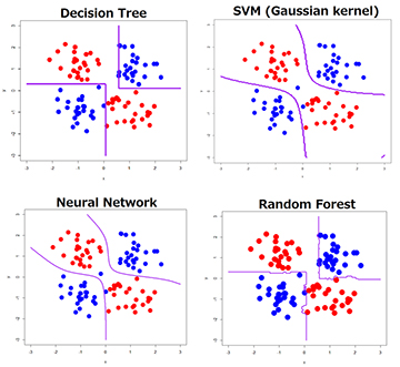
Image By: Data Scientist TJO in Tokyo

Model:
The decision tree is a supervised nonparametric learning method.

Imagine a decision tree like a game of answering ‘if-then’ questions (forks) which define the recursively distribution of data examples under features values. The internal node in each fork asks a feature value; and the branch gives the corresponding value for each example. That value between the branches is called a split point;namely, data to the left of that point are get categorized in a different way than that of the right. The final nodes at the bottom of the decision tree are known as terminal nodes or leaf nodes and they vote on how to classify new data. Each leaf node corresponds to the final output.

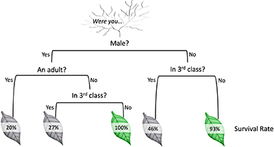
A visualization of a decision tree on titanic data, by Algobeans.com

Algorithm:
Scikit-learn and R implement an optimised version of the CART algorithm.
Other algorithms include C4.5, ID3, CHi-squared Automatic Interaction Detector and Conditional Inference Trees.
Pseudocode:

1. Start with all the data at the root node.
2. Split the training set into subsets, such that the examples with the same output value are grouped together.
3. Scan all the features for the best one to split on.
4. Once found, put it at the root node.
5. Do the split and move downwards.

Repeat step 4 and step 5 until the maximum allowable tree depth is reached where we let the leaf nodes to predict the outcome.

Split means, placing the data into left and right subsets in such a way that examples with the same feature value are groupped together. The split of categorical values is done via Gini, Information Gain, Chi-square, and entropy.

Feature Selection
When interpreting a model, the first question usually is: what are those important features and how do they contributing in predicting the target response? In linear regression this is equivalent of asking which explanatory variables (x) are significant predictors of the dependent variable(y), and how do they impact the latter.
Features that do not contribute to the model’s predictions have to be removed. This helps us to improve the prediction accuracy and to avoid model overfitting and slow training times. In addition to that, we acquire a better understanding of the underlying process that generated the data. Domain experts usually try to find ways for the the model to account for the variability in the changes in the outcome, to ensure generalization.
Methods:
1. Univariate or Filter methods assign scores to the features by looking only at the intrinsic properties of the data. They are scalable and efficient provided that they are computed only once, and then different classifiers can be evaluated.
2. Wrapper methods assess the relevance of a set of features instead of individual features. Different features combinations are compared to other combinations; then based on model accuracy, they assign a score on each combination. It is slower than the filter approach, and becomes even more computationally expensive when there are different models to be implemented.
3. Embedded approaches are far less computationally intensive than wrapper methods, since they learn which features best contribute to the accuracy of the model while the model is being created. These techniques introduce additional constraints into the optimization of a predictive algorithm to bias the model toward lower complexity with fewer coefficients¹.
4. Principal Component Analysis is a dimensionality reduction technique that uses linear algebra to transform the dataset into a compressed form. We have to perform it beforehand to give our tree a better chance of finding the important features.

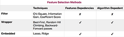
Feature Selection Methods: What techniques usually used by them, do they take into account the potential depedencies among different features and/or their depedence to the algorithm

Individual decision trees intrinsically perform feature selection by selecting appropriate split points. The basic idea is: the more often a feature is used in the split points of a tree the more important that feature is².
In our example,the most important feature stands out for Sex, as we can figure out with features_importances. Usually, we compute feature importances (where all features scores add to 1) and we remove low-scoring features.

Novel application of decision trees

Novel applications of decision trees can be found in image mining like tumor detection and classification in MRI scans and learning human pose recognition in single input depth images.
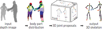
In the latter, the decision tree takes a pixel and classifies the color of it it w.r.t. to the different parts of the body³. The questions it asks are not the same for every pixel and the possible answers are exponential. This results in a less interpetable model since the people behind it are able to just get a sense of what the algorithm is doing intead of knowing exactly how the desicions are taken.
The emphasis of the researchers’ work is not put in the algorithm programming per se but in designing the training set in such a way to capture all the kind of variations.

Following, there are the algorithm’s steps:

1. A single input depth image is segmented into a dense probabilistic body part labeling(training data),
2. Reproject the inferred parts into world space,
3. Localize spatial modes of each part distribution,
4. Generate (possibly several) confidence-weighted proposals for the 3D locations of each skeletal joint.
   

   

The awesome documentary ‘The Secret Rules of Modern Living Algorithms’, a very helpful visual introduction on desicion trees and the references I have listed below, insired me a lot to take these notes.