Matrix Factorization Collaborative Filtering

Photo by: Nathan Dumlao on Unsplash

Recommender systems is a specific type of information filtering technique that attempts to predict information items that are likely of interest to the user. Collaborative Filtering(CF) is the most popular approach in recommender system research.

How Collaborative Filtering works?
Collaborative Filtering builds a model from user’s past behaviour (item based) as well as similar decisions made by other users(user based); then use that model for the prediction. It employs similarity measures either in a neighbourhood search space or in a latent space to extract this information from data.

Thinking CF in terms of Google ranking algorithm?
The most significant difference between them is that the latter finds efficiently web pages in the world wide web whereas the first finds efficiently items like products or movies in a specific application context like Amazon and Netflix.
To put it straightforward, given a user query, the PageRankⁱ algorithm returns an order of web pages such that the one of the top is the one that a user will be more likely interested in. Google search results vary, even on the same device and using the same keyword phrase because of user’s personal search and click history factor.

Different CF working approaches?
Similarly, CF exploits user’s history by using

• heuristic models (based on Pearson/Cosine/Jacquard functions that compute pair-wise similarities)
  • item-based neighbourhood: find item i that is similar to k items which users has bought/search for/click to.
  • user-based neighbourhood: user A bought items 1,2,3 and user B bought items 1,2,4. User A will likely buy item 4.
• factor models (based on mathematical techniques that infer factors by minimising the reconstruction error based on observed data.)
  • matrix factorization: finds hidden similarity layer between the users and the items
• hybrid models

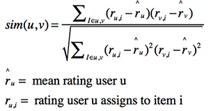
Pearson correlation computes similarity between users v and u

In this post, you’ll read about:

• What is the intuition of Matrix Factorization?
• How it works?

Matrix Factorization is a learning algorithm belonging to latent factor models and has been used in many machine learning applications like training deep networks, modelling a knowledge base and recommender systems. It allows for:

1. solving linear equations
2. compressing data
3. transforming data

1
2

Matrix Factorization is now a popular baseline in recommendation algorithms 
since it outperforms other state-of-the-art collaborative filtering techniques.

Let’s go a step behind and remember our schooling years in math class.
Factorization means decomposing an entity into multiple entries - that can be typically ‘managed’ more easily. For example, 8 is the product of 4 and 2.

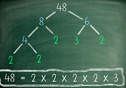
Image Source: Science ABC

1
2
3
4
5
6
7
8
9
10
11
12

Process:
This problem is solved in two steps:
1. decompose the rating matrix to model both users and items 
as coordinates in a low dimensional feature space
i.e. each user and each item has a feature vector, and
2. compose an approximation of the rating matrix by computing the inner product
 of the corresponding user and item feature vectors, to predict the rating.
Each rating represents the interest of a user to an item and 
both oserved and unknown ratings are modelled as step (2) indicates.

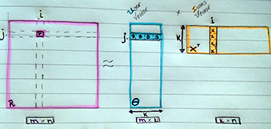
Factorizing the Rating Matrix (R) into the inner product of User (Θ) and Item (X) Matrices
Each rating of user θ_j on item x_i is modelled as the inner product of them: r_ji = x_i^T θ_j

1
2
3
4
5
6

Given:
m training examples =  [users, items, ratings]
n features(number of columns of original rating matrix)
Goal:
Predict the ratings in the test data set by minimizing the cost function.

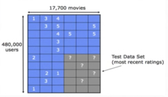
A set of training and test examples represented as a sparse matrix

So, assuming R is a matrix of users rating items, it is pretty straightforward to assume that each item is tied to one or more categories with some strength, each user likes/dislikes some item-categories with different strengths, and the rating that a user should have given an item depended on the similarity between their characteristics and this item’s characteristics.

Learning Algorithm
Model Training:
Convert matrix factorization to an optimisation problem & minimise cost function

Optimization Objective:
In each step, we are solving a regularized least square problem:

1. Fixⁱⁱ the user feature vector, and solve for the item feature vector
2. Following that, fix item feature vector mj, and solve for user feature vector.
3. Simultaneously minimize the cost function J and update the values of user & item feature vector using Gradient Descent
   Repeat this process until convergenceⁱⁱⁱ

The first term in the following cost function J, is the Mean Square Error (MSE); and the second term is the regularization term added to prevent overfitting.
The following function says: ‘For all the observed ratings(R^ji!=NA) compute the difference between the original rating matrix R and its approximation(R - Θ^T * X), then update the latent feature vectors of users and items.

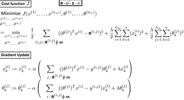
Simultaneous Minimization of Cost Function J and Gradient Update, by Andrew NG ^iv

To monitor convergence, we plot J and number of iterations and make sure its decreasing. The learning rate α decides how fast the gradient will step forward. To choose an optimal value for a, we can

1. try a number of different value ranges,
2. plot J with the number of iterations
3. choose the one that decreases J.
   If gradient descent decreases quickly, α is efficient.

Some final notes
Apart from trying to produce a minimal value of this cost function for a given k(effects) and λ(regularization), it is essential to determine what are the optimal values for those parameters.
Large values for λ results in high bias, namely data do not fit the model while small values for λ results in high variance, namely themodel fails to generalize as new data come. We can compute different values for λ and after plotting cost function, pick the one that decreases the cost function.
Another idea is to incorporate Cross Validation or another more sophisticated optimization process to ensure a good value selection for those parameters.
Gradient descent works well in optimizing MF models only when the dimensionality of the original rating matrix is not high; as otherwise there would be many (nk + mk) parameters to optimize.
Bear in mind that introducing distributed computing could alleviate this problem.

An alternative to simultaneous optimization, is to use Alternating Least Squares which 2-teration process. In ALS, we solve a linear regression problem with the difference we do not have fixed weights. To put it differently, we solve for x given θ, compute gradient x (step 1), then we solve for θ given x, compute gradient θ (step 2) and we iterate. ALS to converge slower.

Another thing to keep in mind is that, imposed constrains shape the factorization and yield different views on data. Constrains are all the possible values variables may take.

Concluding, there are many FM techniques in which PCA and SVD are considered as baseline. Non negative MF and Probabilistic MF are also well-known MF tachniques.