Diving Into Neural Networks

Photo by: David Bruyndonckx on Unsplash

Understanding Artificial Neural Networks without burning your Brain Neural Networks

‘If you don’t challenge your brain, nobody else will.’

BNN Learning
When we think about training a machine to learn, what is more natural than to think of our brain as a complicated learning machine. Besides, the first work that is now generally recognized as AI (1943) drew knowledge of the basic physiology and function of neurons in the brain ¹. Neural Networks are a major area of research in both neuroscience and computer science.
Before diving into how Artificial Neural Networks(ANN) learn, let’s explore something more familiar: how the brain learns.

A biological neural network(BNN) is a collection of neurons (electrically excitable cells) connected together through synapses that processes and transmits information. A group of neurons forms a “distributed-database”ⁱ of encoded information such as skills, thoughts and feelings and other long-term memories.

Ok, but how the brain learns?
According to neuroplasticity², the brain can change in three very basic ways to support learning:
1.Chemical: transfer chemical signals between neurons. It supports short-term memory.
2.Structural: altering/creating the connections between neurons. It supports long-term memory.
3.Functional: The more we use a brain region, the more excitable and easier is to use it again and again.

“Behaviour drives changes in the physical structure of the brain which manifest as changes in our abilities.”

ANN & BNN Learning Costs
BNN learning is an expensive problem due to the cost related with the information load, the very large doses of practise that are needed. Generally we humans unconciously decide to learn a new skill after evaluating the function of f(x) = y where we put the following variables as input
i. effort,
ii.time,
iii.cost against other choices that our time and/or efforts could be spent on,
and take as output the learning decision.

Learning is best when you connect it to things that you’ve already learned. We’ll make a connection between the known (BNN) and unknown information by diving into an artificial feedforwardⁱⁱⁱ neural network, named Ceniaⁱⁱ.
Cenia’s learning was earlier a really expensive problem due to the lack of data and the slow computers; now both of the sources are available.
The learning cost of a neural net is related to efficiency and accuracy. Efficiency cost is about the computational resources like the training time, the complexity of the model and the memory space needed for the model to run. Accuracy is related with how close to the truth is the prediction result. Usually measured via mean squarred error and the ROC learning curve.

“Every luxury has a cost, and everything is a luxury, starting with being in the world.” –Cesare Pavese

Problem Formulation: Classify Images

Let’s say the desired learning outcome of Cenia is to detect which photos contain a duck. This is a classification problem because the output variable is a discrete value and not a continuous one.

1
2
3

y = {0,1}
0: not a duck
1: a duck

Let’s see how our brain can process images before teaching Cenia to do that. One of the brain’s earliest visual processing centers, V1, identifies simple forms like vertical, horizontal, and diagonal edges of contrasting intensities, or lines. Downstream visual centers V2, V3, V4 weave together these basic visual forms to create the beginnings of a visual tapestry³. The human brain does so in a fraction of a second and automatically organize information into a “whole” even as an individual’s gaze and attention are focused on only one part⁴.

“An image can be compared with a bag of thousands of little Lego blocks in chaotic order.”

ANN Learning
Cenia’s learning can be achieved through three steps:

1. Build
2. Train
3. Test

Let’s decompose each step and then see the big picture (bottom-up approach). So, do not worry about concepts that you don’t grasp right now because everything takes shape later.

1. Build the model: Architecture

In the building step of a supervised classifier, we have to decide about the training set, the data preparation and the model architecture.

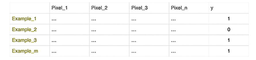
The number of training examples are m and of features for each training example is n.
The columns’ values of the matrix represent the nodes in the input layer
The values of column y represent the nodes in the output layer.

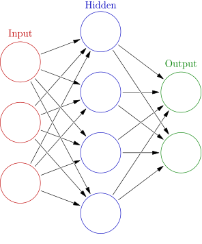
A sequence of integers describes the number of nodes in each layer. The network above is a 3-4-2.

Feedforward Function
Each neuron of the layer is like a function, it takes an input and returns an output. Each layer, except for the input layer, produces an output by applying a function to the output of the previous layer. So, the output of the previous layer is the input for the next layer. In this way, each layer gets you farther from the raw pixels and closer to your ultimate goal.

Each synapse of each layer firstly apply a linear transformation to the data in order to create weights (W) for each input (aka coefficient multipliers), as the following equation shows:

1

z = W*X or f(x) = W*X (1)

After summing (1) for each input, each neuron of the hidden, and later output layer, applies a non-linear squashing function like sigmoid, known as activation function. Activation functions squashe the values in a smaller range, i.e. sigmoid neuros return values between 0 and 1.

1

a = f(z) or g(f(x)) = 1/(1+exp(-W*X)) (2)

So with one hidden layer, the above functions happen two times each, since we have two ‘blocks of synapses’. At the begging, each synapse is assigned with a random weight W.
To put it simply, the output is computed by multiplying the input (x) by the weight (w) and passing the result through some kind of activation function.

Input Layer → x: look for edges (Lego blocks) in the raw pixel data
The input layer will always be equal to one. The number of neurons comprising that layer is equal to the number of features (columns) in our input data. So if each training example, namely each image is represented by 200 floating point numbers (pixels), then the nodes in the input layer will be 200. One additional node is added sometimes for a bias term. The “bias” nodes are like intercept terms in regression. They ensure that even if all the inputs are zero, there will be an activation in the neuron. Bias indicate the direction of the activation function whereas weights indicate the steepness of the activation function.

Hidden Layer → f(x): compose edges (Lego blocks) for detection of the features we egineered (tapestry)
For the large majority of problems, one hidden layer is sufficient. The more hidden layers are added to a neural net, the harder is to be trained but when complex problems is the case the more accurate the model become.
The hidden layer captures the significance of each input and transfer it to the output layer . The significance of each input depends on the weights values. Consider for instance:

1
2
3

z = 5x, W =5
z = 3x, W =3
The first input is more significant than the second.

Cenia will tell us if there’s a duck in a picture, if we give her the right tools to give an order on the Lego blocks of the picture. Every AI system needs a semantic understanding of the world to be able to take further actions.
So besides the features (pixels) we explicitly have as part of the raw image, we should engineer the other features that we implicitly have for the specific problem learning. Our duck detector is made up of different physical features like leg detector (to help tell it’s a bird) and a body detector (since the duck is shaped like a horizontal rectagular) and a bill detector (to tell it’s too big to be a duck). Suppose these are the three elements of our hidden layer: the features we engineered to help identify ducks. Keep in mind that there is no magic formula for selecting the optimum number of hidden neurons. Sometimes the number of nodes of the hidden layer are computed by the mean of input and output nodes or through other thumb rules, as shown below:

1
2
3
4
5

h = number of hidden neurons
i = number of input neurons.
o =  number of output neurons.
e = number of examples in training data set.
αα = an arbitrary scaling factor usually 2-10.

1

h = sqrt(i*o)

1

h = e/(a*(i+o))

Output Layer → g(f(x)): compose the edgineered features of the previous layer to get our final answer
The output layer will always be equal to one. The number of neurons comprising that layer is equal to the number of outputs we expect. Here, we have two nodes since we have two labels (0,1). When the leg, body and bill detector from the previous layer turn on with the right patterns, the answer will be 1 (a duck). Otherwise will be 0.

• Cenia: ‘Was I correct?’
• We: ‘No’
• Cenia: ‘So I was not properly taught’

Cenia’s answers by now will be far away from the truth. She has not yet learned to recognize ducks because we haven’t trained her yet.

2. Train the model: Minimize the Cost

Training a network means minimizing the cost function;
Minimizing the cost means changing the weights W of our model.

To improve Cenia’s predictions we need to quantify how wrong her answers are. We’ll do that through the cost function. We compute the cost function for each input with different weight values until we find the weight values that minimize the cost. The cost is the difference between the real value y (from the training data) and the predicted output h (from the feedforward method). Let’s assign at variable h the predicted output of the third layers’ activation funcion f(g(x)).

1

J = 0.5 * sum ((y-h)^2) (3)

‘Cost Function imitates our Conscious Function, providing that Conscious aims to understand reality as close to the truth as possible.’

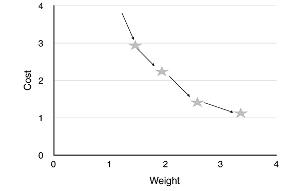
We need to find the change rate of the cost function(dJ) so as to select the direction that goes downhill. This would save us time because it would prevent us from searching of weights values that increase the cost^iv, namely going uphill.

1

dJ/dW : the change rate of J with respect to W

Change rate = Slope = Steep = Derivative^v = Gradient Descents => Find the values of Weights that minimize J

To estimate the values of W, we compute Gradient Descents for each weight. Gradient descents is about finding the change rate of J with respect to W and choosing the Weight that minimizes J. After summing up the gradients, we decide the next step of the function dJ/dW. In the diagram below, the step is the star.

Backpropagation Error → g(f(x))’

Now that we have find the costs and the weights, we should transfer them back to the input layer to perform the forward function again with the found values. The weights that contribute more to the error, would have larger activations and would be changed more when we perform Gradient Descent.
This procedure ‘transfer the weights forward w.r.t. x - transfer the error backward w.r.t. y’ would iteratively runs until we find the optimum values for our weights. In this way, Cenia would be able to predict most of the pictures correctly.
The backpropagation error is called delta. After we compute the activation function (2) for a node of output layer, delta for this node would be equal to:

1
2

d3 = a - y       (4)
dJ/dW2 = a * d3  (5)

where y is the real value of the output.
The error for the previous layer would be slightly different:

1
2

d2 = (W2*d3) * a'  (6)
dJ/dW1 = X * d2    (7)

where a would be the activation function of hidden layer and a’ would be its derivative. We have no d1 because the first layer corresponds to inputs.
Note that, in (5) ‘a’, in (6) ‘W’, and in (7) ‘X’ would all be transposed matrices; since we want to make matrix multiplication along the training examples. What is missing from this post, is the linear algebra like matrix multiplication and transposes that lie behind these functions. But to keep things simple and not to burn our brain neural nets we talked only about the notion of neural networks and not the maths behind it.

Would you like to apply neural nets to code and also check the maths? See this repo on github.
Or would you prefer to learn more on ANN and computer vision? See this and this video.
Get more background on the way our brain learns in this ted talk.

Notes: