Parallel Computing on Big Data

Image by Joshual Sortino

With the advent of Big Data, the interest towards distributing and parallel computing from both academia and industry has grown even more. These concepts come handy to people that develop algorithms on large-scale data or use cloud architecture for computationally intensive problems. For everyone who participate in a project development team, it would be helpful to know the fundamental of these computing paradigms in order to understand both the efforts and strengths that characterize a scalable product. I am not saying that distributed architectures are the bless holy for every project, on the contrary there are problems where distributed architectures are not required at all.

In this post, you’ll read about:

What is scalability in big data?
What are some applications that need parallelism?
What is parallel machine learning?
What is the difference between distributed and parallel computing?
Why MPI is inefficient towards big data problems?
What is the value of Map Reduce framework?
How Map Reduce works?
What is the trade-off between communication & computation cost?

To address the scalability issue and accelerate tasks in Big Data problems, data processing and analysis must be carried out by parallel and distributed programming models.

But what does scalability means anyway?

Scalable is considered an algorithm, a design, a networking protocol, a program, or other system that fulfills the following criterion:
it is able to still have high performance in case when one ‘large’ thing from the below happens:

1. input a large dataset of data points or attributes to the system
2. output a large dataset of data points or attributes from the system
3. connect to the application a large number of users/a large number of compute nodes
4. a large number or parameters required for the method to be build

Two examples that require parallelism are ¹:
i. The ranking of Web pages by importance, which involves an iterated matrix-vector multiplication where the dimension is many billions.
ii. Searches in “friends” networks at social-networking sites, which involve graphs with hundreds of millions of nodes and many billions of edges.

Examples of methods that often take the advantage of parallelism and distribution include document clustering, web log analysis, machine learning and pattern-based searching and sorting.

To make things more concrete, let me show you a simple example of a parallel machine learning algorithm. We have 180.000.000 training examples that we want to use in order to train a logistic regression classifier. But such data cannot run on one conventional computer. What do we do? Let’s say we are so lucky that we have in our house the new iMacPro which has 18-core processors. We divide the training set equally in so many chunks as the processors we have. Thus each chunk now has 10.000.000 training examples which are fed into each of these cores. Each one simultaneously runs the algorithm and give their answer asynchronously when they end up the calculations. Then, we take each result and combine them to finish our training. In this way, we achieve a speed up of almost 18x. This is called parallel machine learning because the computations run in a single machine in the form of mutli-core processors.

On distributed computing, we follow the same procedure with the difference that these data training chunks are fed across on multiple computing machines instead on multiple cores at the same machine. Even if you with your team desire to develop the most sophisticated deep learning system you can now make use of NVIDIA DGX-1 whose GPU architecture is designed for AI. Mind that, the advantage of multicores against multiple machines is that we do not have to worry about network issues such as network latency.

MPI was until recently the common parallel programming model for data analysis. But challenges such as big data access (since they are often stored in different locations), non-robust fault-tolerant mechanism (since big data jobs are time-consuming) and the need for an extremely large main memory to hold all the preloaded data for the computation (e.g. in a data mining problem all the data have to be available at the memory from the start) made it inefficient ². These issues are partially been overcame through Map Reduce invention.

Hadoop, Map Reduce and NoSQL are the major technologies in big data management. Map Reduce has become a dominant parallel computing paradigm for big data processing. But why? What we achieve by using it?
It achieves fast computation and automatically parallelization of colossal datasets processing via using hundreds or even thousands of commodity machines (aka a distributed system). A MapReduce algorithm instructs these machines to perform a computational task collaboratively. It can be used on multi-core system architectures or dynamic cloud environments as well.

How Map Reduce works?

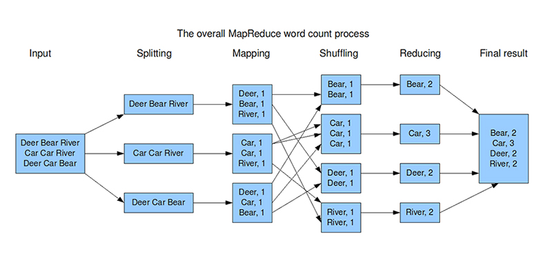
Initially, the input dataset, which is treated as a collection of elements (e.g. documents, tuples etc), is splited into key-value pairs (chunks) to allow composition of several MapReduce processes. Note that, the keys are not relevant and we shall tend to ignore them. After the distribution of chunks to machines, map reduce algorithm executes four phases on rounds or otherwise called jobs:
i. map-mappers: each machine prepares the information to be delivered to other machines
ii. shuffle: takes care of the actual data transfer from mappers to reducers.
iii. sort: tell to reducer when to start a new reduce task. A reducer task starts when the next key in the sorted input data is different than the previous.
iv. reduce- reducers: receives a list of a key and its list of associated values. The outputs from all the reduce tasks are merged into a single file.

The first two phases enable the machines to exchange data. Shuffling can start even before the map phase has finished, to save time for mapping. Sorting on the other hand saves time for the reducer. No network communication occurs in the reduce phase, where each machine performs calculation from its local storage. The current round/job finishes after the reduce phase.
The below graph, made by Xiaochong Zhang, shows the execution of MapReduce process on word counting. Mind that, at the illustration, the phase of sorting, which is not depicted, is in the same column of shuffling.

Ideally, a MapReduce system should achieve a high degree of load balancing among the participating machines, and minimize the space usage, CPU and I/O time, and network transfer at each machine. However, again when designing map reduce algorithms there are concerns about communication cost. The decision one has to make when using map reduce is to choose the trade-off between computation and communication cost. The communication cost and computation cost can be measured as ²

1
2
3

Communication cost = total I/O of all processes.
Elapsed communication cost = max of I/O along any path
Elapsed computation costs analogous, but count only running time of processes.

To refine the explanation, say that

1
2
3
4

the communication cost is the sum of 
input file size + 
2 × (sum of the sizes of all files passed from Map processes to Reduce processes) + 
the sum of the output sizes of the Reduce processes

whereas

1
2

the elapsed communication cost is the sum of 
the largest input output for any map process,plus the same for any reduce process.

In bottom line, parallel execution of processing is essential for big data problems because scalability and time are two crucial and highly related issues, since we are talking about analysis of terabytes data sizes. Map Reduce is the dominant distributed framework used to process big data. For diving deeper into these concepts I recommend checking the informative two sources listed below. Additionally, for those who want to become ‘distributed-geeks’, I myself inveted this magnificent term 😯 , a collection of books, papers, cources etc are made by Abhishek L